|
Economic Order Quantity (EOQ) models are the most basic models of
inventory management. The approach in EOW models is essentially to
trade-off various relevant costs and derive an order quantity and time
for placing an order such, that the total costs are minimized. This
note discusses the basic EOQ model and the sensitivity of costs in EOQ
model to various parameters. Later an extension of basic EOQ model is
discussed in which case back-orders or shortage are allowed.
1.1 Functions
of inventory
Though inventory is an idle
resource, it is almost essential to keep some inventory in order to
promote smooth and efficient running of business.
Consider the case – an enterprise that does not have any inventory.
Clearly, as soon as the enterprise receives a sales order, it will
have to order for raw materials to complete the order. This will keep
the customers waiting. It is quite possible that sales may be lost.
Also the enterprise may have to pay high price for some other reasons.
On the other hand, inventory may promote sales by reducing customers
waiting time. It is essential to maintain the inventories in
order to enhance stability of production and employment levels.
Consider the case of seasonal items. Any fluctuation in demand can be
met if possible, by either changing that part of production or with
inventories. However, if the fluctuation .... is not by changing the
rate of production, one has to take into account the following cost.
|
|
Cost of
increasing production and employment level:
(i)
Employment and training
(ii)
Additional staff and
service activities
(iii) Added shifts
(iv) Overtime
costs
Cost
of decreasing production and employment level:
(i)
Employee
compensation
(ii)
Other employee costs
(iii)
Staff, clerical and service
activities
(iv)
Total time costs
|
In other words, the use of seasonal inventories can often ... after
balance of these costs. Broadly, some other functions of inventories
are to :
(i) protect against unpredictable variations (fluctuations) in
demand and supply
(ii)
take the advantage of price discounts by bulk purchases
(iii) take the advantage of batches and longer production run.
(iv) provide flexibility to allow changes in production plans in view
of change in demands, etc. and
(v) facilitate intermittent production.
Elementary Inventory Models (with Deterministic Demand)
Let us consider the inventory models in which demand is assumed to be
fixed and completely pre-determined.
Notations
D - annual demand rate
V - unit purchase cost or unit cost of production (Rs./unit)
A - ordering or set up cost (Rs/order)
R - holding cost per Rs. per year (*Rs./Rs/year) (Inventory carrying
charges factor)
B - shortage cost per Rs. short unit time (Rs/ Rs/ year)
Q - order quantity (to be determined)
See Inventory numericals here
Inventory Cost
The heart of inventory analysis resides in the identification of
relevant costs. Some of the important costs that apply to inventory
situation are :
Ordering or
set up costs
These are costs associated with ordering or manufacturing goods
through purchasing or manufacturing and are known as set up costs or
cost of ordering. Set up costs are generally assumed to be independent
of the quantity ordered or produced.
Purchase cost
or production cost
When large production runs are in process, these results in reduction
of production cost per unit. Often, discounts are offered for the
purchase of large quantities. In other words, often the unit cost of
an item depends on the quantity procured or produced.
Inventory
Holding Cost
The cost associated with carrying or holding the goods in stock are
known as carrying or holding costs. These costs arise due to the
storage costs, property taxes on the items in inventory, interest on
the invested capital (interest on value of the inventory items,
spillage of the inventory items, depreciation of the inventory items,
transportation and handling of the items in inventory, etc.
Shortage or
stock out costs
The costs that are incurred as a result of running out of stock are
known as stock PUT TO SHORTAGE COSTS. As a result of shortages, sales
or goodwill may be lost. If the unfulfilled demand for the items can
be satisfied at a later date (back order case), in this case cost of
back orders are assumed to vary directly with the shortage quantity
(in rupee value) and the delaying time (Rs./ Rs.) . However, if the
unfulfilled demand is lost (lost-sales case), in this case cost of
shortages are assumed to vary directly with the shortage quantity (Rs./
unit shortage).
Inventory
Models
1. Economic Lot size or Economic Order
Quantity Model
Assumptions :
1) The rate of demand for the item is deterministic and is a
constant D units per per annum, independent of time.
2) Production rate is infinite, i.e production is instantaneous
3) Shortages are not allowed
4) Lead time is zero or constant independent of demand and the
quantity ordered.
5) The entire quantity is delivered as a single package (or production
in a single run).
Objective :
To minimise the average annual variable cost.
Problem :
To determine when an order should be placed and how much
quantity should be ordered.
The annual variable costs for this problem are two types - 1) ordering
or set-up cost and 2) Inventory holding cost.
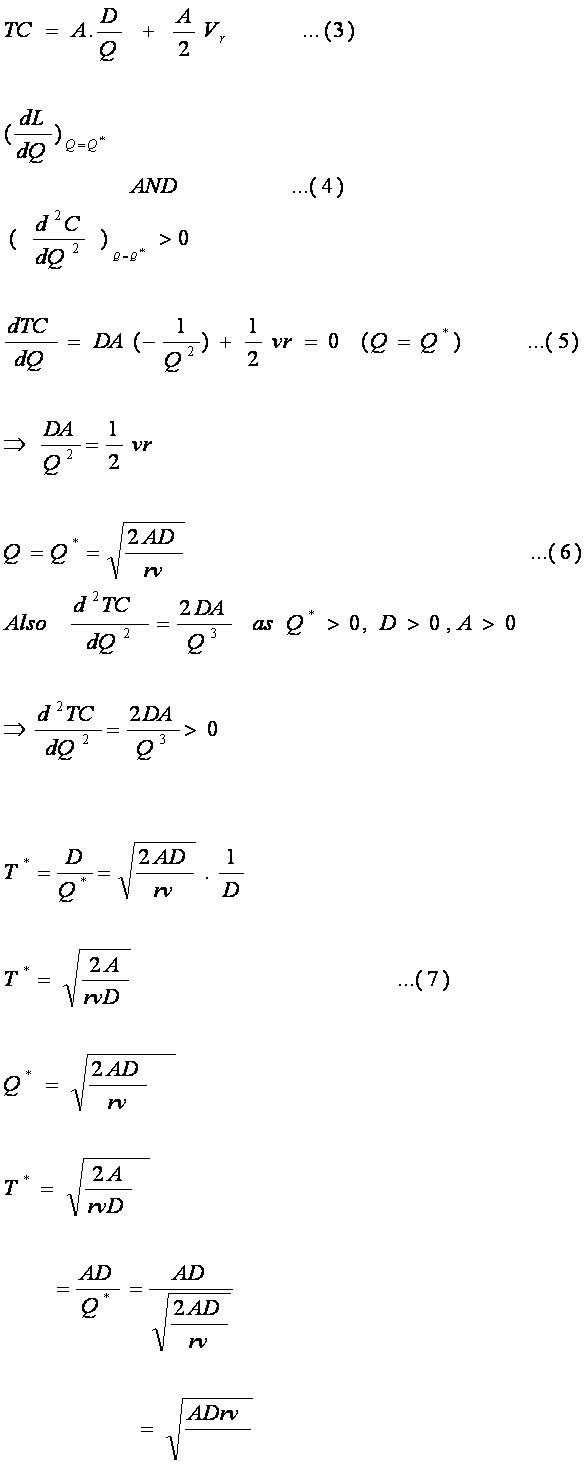
As Q is the order quantity and D is the annual demand, the number of
orders per years will be D/Q. Therefore, the annual ordering cost will
be = A.D/Q ........ (1)
Elementary Inventory Models
(with Deterministic Demand)
Let us onsider the inventory models in which demand is assumed to be
fixed and completely pre-determined. The inventory models with
uncertain demand are considered later.
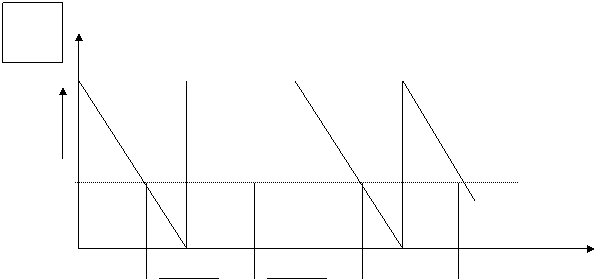
and leadSince quantity Q is ordered every
time an order is placed and since the rate of demand is D, the time
between two successive orders (T) will be 0/0. teh figure 1 shows the
inventory level Vs Time rotationship.


Time
From Fig.1 it is obvious that since the inventory is
consumed at uniform rate and since maximum inventory level is Q, the
averaghe inventory will be Q/2.
Hence, Average Investment in Inventory will be = Q/2.v
And the average Inventory Holding Cost will be = Q/2. ve .... (2)
Hence the total annual variable cost (TC) = ordering cost + Inventory
Holding Cost.


The relationship between order quantity and
(1)
Annual ordering cost
(2)
Inventory Holding cost
(3)
Total Annual Cost 
   Is given in Figure 2
Total cost = TC
Average Inventory Holding
Cost = Q/2. vr
TC *
 AnnualorderCosts=D/Q.A AnnualorderCosts=D/Q.A
0
Q *
Economic Order Quantity and Reorder
Level with Fixed Lead Time
In the above discussion and in figure 1 are considered that load time
is zero. However, if lead time is constant the above results can be
used without any modification.
If lead time is say constant and equal to L (in years) then during
lead time, consumption is LD units. This élans that as soon as the
inventory Q level reaches LO units, a new order will have to be
released for Quantity G*, the new order will arrive exactly
after time period L at which time inventory level will be zero and the
system will repeat itself. The inventory level at which the order is
released is known as reorder level (R=0) i.e. Rp=LD. (Figure 3 shows
the inventory level vs time the constant lead time situation.
See Inventory numericals here
   
4.3 Properties
of EOQ model and Sensitivity Analysis
In the above nodal, various parameters are used such as demand (D),
inventory carrying charges factor (r), ordering or set-up cost (A).
These parameters are estimated and though they are assumed to be
known, in real life what we have is an estimated value which may be
different than real value for various reasons.
For this reason it is important for practical purposes to test the results
of the EQQ model and find how sensitive the results are to the changes
in various parameters.
The sensitivity can be explored in various ways. Let the “true” rate
of demand is D, “ true” value of order cost is A, “ true” value of
inventory holding cost is r and “true” value 9of unit purchase cost or
production cost is v. Then the “true” optimal value of order quantity
(Q*) will be, (be eqn. 8),


There

 
In
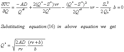
case when shortage costs are infinitely high (i.e. when shortages are
not allowed) b = ¥ and eqn. 17 will reduce to
 Which is same as equation (6), i.e.
optimal order quantity for the E0-model. This is obvious since the EOQ
model assume that no shortages are allowed which imply that the
shortage are infinite.
See Inventory numericals here
|